This paper proposed a theoretically plausible dropout method for RNNs. When applied to language modeling, the new technique outperforms existing approaches.

Introduction

Dropout is a popular regularization technique which prevents deep networks from overfitting. But empirical results have shown the negative effects of applying dropout in RNNs' recurrent connections. Only dropout in non-recurrent connections has been shown to improve performance. So, people often believe that noise added to recurrent layers will be amplified across long sequences which drown the signal.

The authors proposed a new dropout variant, which repeats the same dropout mask at each time step, at each layer, for both inputs and outputs, as shown in Figure 1:

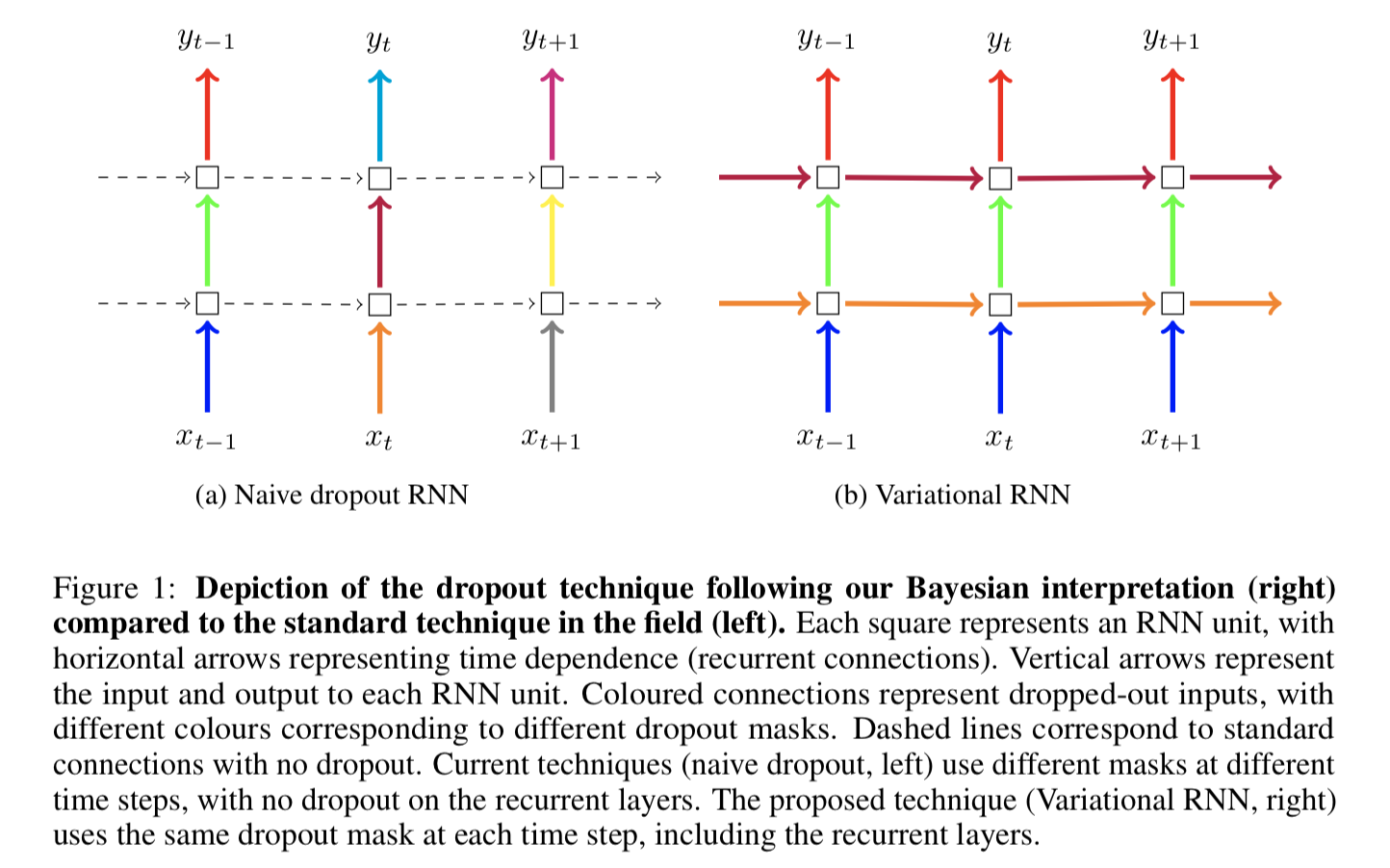
For figure to the right, blue connects share the same dropout mask, then green ones, then red ones. Those dropout masks are in fact dropping recurrent units (words) out. Differently, the purple and yellow masks are applied to hidden states across time steps.

Background

This variant is variational inference based, what does this mean?

Bayesian Neural Networks

In Bayesian regression, given data inputs \(\mathbf{X} = \{ \mathbf{x_1}, \cdots, \mathbf{x}_N \}\) and outputs \(\mathbf{Y} = \{\mathbf{y}_1, \cdots, \mathbf{y}_N\}\), we want to find the parameters \(\omega\) which are likey to have generated that data. Following the Bayesian approach, we put some prior distributions \(p(\omega)\) over the parameter space.

The likelihood distribution \(p(\mathbf{y} | \mathbf{x}, \omega)\) for classification is:

\[p(y = d|{\mathbf{x}},\omega ) = {\exp (f_d^\omega ({\mathbf{x}}))/\sum\limits_{d'} {\exp } (f_{d'}^\omega ({\mathbf{x}}))}\]

The authors wrote a different equation:

\[p(y = d|{\mathbf{x}},\omega ) = {\text{Categorical}}\left( {\exp (f_d^\omega ({\mathbf{x}}))/\sum\limits_{d'} {\exp } (f_{d'}^\omega ({\mathbf{x}}))} \right)\]

I don't know what does that mean.

Anyway, the posterior distribution over parameter space \(p(\omega \vert \mathbf{X}, \mathbf{Y})\) is then used to predict a new input point by integrating

\[
p({{\mathbf{y}}^*}|{{\mathbf{x}}^*},{\mathbf{X}},{\mathbf{Y}}) = \int p ({{\mathbf{y}}^*}|{{\mathbf{x}}^*},\omega )p(\omega |{\mathbf{X}},{\mathbf{Y}}){\text{d}}\omega
\]

If you place a prior distribution over a neural network's weights, then that NN is called a Bayesian NN. The common approach is to place gaussian prior \( p({{\mathbf{W}}_i}) = \mathbb{N}({\mathbf{0}},{\text{ }}{\mathbf{I}})\) over weights, to assume point estimate for the bias.

Approximate Variational Inference in Bayesian NN

What's Variational Inference

Given dataset, the posterior over parameters \(p(\omega\vert \mathbf{X}, \mathbf{Y})=\frac{p(\mathbf{X},\mathbf{Y}, \omega )}{p(\mathbf{X},\mathbf{Y})}=\frac{p(\mathbf{X},\mathbf{Y}\vert \omega)p(\omega )}{\int p(\mathbf{X},\mathbf{Y}\vert \omega)p(\omega ) \text{d}\omega }\) is not tractable. The denominator integrates over entire parameter space. To approximate, we find a tractable \(q(\omega\vert \mathbf{X}, \mathbf{Y})\), and minimize the KL divergence between \(p(\omega\vert \mathbf{X}, \mathbf{Y})\) and \(q(\omega\vert \mathbf{X}, \mathbf{Y})\).

KL divergence

\[\begin{equation} \begin{aligned}
{\mathbf{KL}}(q(\omega )||p(\omega |{\mathbf{X}},{\mathbf{Y}})) &= - \int q (\omega )\log \frac{{p(\omega |{\mathbf{X}},{\mathbf{Y}})}}{{q(\omega )}}d\omega \hfill \\
&\propto - \int q (\omega )\log \frac{{p({\mathbf{Y}}|{\mathbf{X}},\omega )p(\omega )}}{{q(\omega )}}d\omega \hfill \\
&\propto - \int q (\omega )\log p({\mathbf{Y}}|{\mathbf{X}},\omega )d\omega - \int q (\omega )\log \frac{{p(\omega )}}{{q(\omega )}}d\omega \hfill \\
&\propto - \int q (\omega )\log p({\mathbf{Y}}|{\mathbf{X}},\omega )d\omega + {\mathbf{KL}}(q(\omega )||p(\omega )) \hfill \\
&={ - \sum\limits_{i = 1}^N {\int q } (\omega )\log p({{\mathbf{y}}_i}|{{\mathbf{f}}^\omega }({{\mathbf{x}}_i})){\mathbf{d}}\omega + {\mathbf{KL}}(q(\omega )||p(\omega ))}
\end{aligned} \end{equation} \]

Variational Inference in Recurrent Neural Networks

Given input sequence \({\mathbf{x}}{\text{ = [}}{{\mathbf{x}}_1}{\text{, ..., }}{{\mathbf{x}}_{\text{T}}}{\text{]}}\) of length \(T\), GRU is such a repeated application of function \(\mathbf{f}_{\mathbf{h}}\):

\[
{{\mathbf{h}}_t}{\text{ }} = {\text{ }}{{\mathbf{f}}_{\mathbf{h}}}({{\mathbf{x}}_t},{\text{ }}{{\mathbf{h}}_{t - 1}}) = \sigma ({{\mathbf{x}}_t}{\text{ }}{{\mathbf{W}}_{\mathbf{h}}} + {\text{ }}{{\mathbf{h}}_{t - 1}}{\text{ }}{{\mathbf{U}}_{\mathbf{h}}} + {\text{ }}{{\mathbf{b}}_{\mathbf{h}}})
\]

Then the model output can be defined as a affine transform of the last hidden state:

\[
{{\mathbf{f}}_{\mathbf{y}}}({{\mathbf{h}}_T}) = {{\mathbf{h}}_T}{{\mathbf{W}}_{\mathbf{y}}} + {{\mathbf{b}}_{\mathbf{y}}}
\]

To view the GRU as a probabilistic model, we treat \( \omega = \{ {{\mathbf{W}}_{\mathbf{h}}},{{\mathbf{U}}_{\mathbf{h}}},{{\mathbf{b}}_{\mathbf{h}}},{{\mathbf{W}}_{\mathbf{y}}},{{\mathbf{b}}_{\mathbf{y}}}\} \) as random variables. Denote that \({\mathbf{f}}_{\mathbf{y}}^\omega = {{\mathbf{f}}_{\mathbf{y}}}\) to clarify the dependency on \(\omega \).

Use variational inference with distribution \(q(\omega)\) to approximate posterior over \(\omega\). Evaluate each sum term in eq. (2):

\[\begin{equation} \begin{aligned}
\int q (\omega )\log p({\mathbf{y}}|{\mathbf{f}}_{\mathbf{y}}^\omega ({{\mathbf{h}}_T})){\mathbf{d}}\omega &= \int q (\omega )\log p({\mathbf{y}}|{\mathbf{f}}_{\mathbf{y}}^\omega ({\mathbf{f}}_{\mathbf{h}}^\omega ({{\mathbf{x}}_T},{{\mathbf{h}}_{T - 1}}))){\mathbf{d}}\omega \hfill \\
&= \int q (\omega )\log p({\mathbf{y}}|{\mathbf{f}}_{\mathbf{y}}^\omega ({\mathbf{f}}_{\mathbf{h}}^\omega ({{\mathbf{x}}_T},{\mathbf{f}}_{\mathbf{h}}^\omega (...{\mathbf{f}}_{\mathbf{h}}^\omega ({{\mathbf{x}}_1},{{\mathbf{h}}_0})...)))){\mathbf{d}}\omega \hfill \\
\end{aligned} \end{equation} \]

Apply Monte Carlo integration with one singe sample:

\[
\approx \log p({\mathbf{y}}|{\mathbf{f}}_{\mathbf{y}}^{\hat \omega }({\mathbf{f}}_{\mathbf{h}}^{\hat \omega }({{\mathbf{x}}_T},{\mathbf{f}}_{\mathbf{h}}^{\hat \omega }(...{\mathbf{f}}_{\mathbf{h}}^{\hat \omega }({{\mathbf{x}}_1},{{\mathbf{h}}_0})...)))),{\text{ }}\hat \omega \sim q(\omega )
\]

Here we have only one sample, so \(q({\hat \omega})=1\).

Plug this estimator into eq. (2), our minimization object becomes:

\[
\begin{array}{*{20}{l}}
\mathcal{L}&{ \approx - \sum\limits_{i = 1}^N {\log } p({{\mathbf{y}}_i}|{\mathbf{f}}_{\mathbf{y}}^{{{\hat \omega }_i}}({\mathbf{f}}_{\mathbf{h}}^{{{\hat \omega }_i}}({{\mathbf{x}}_{i,T}},{\mathbf{f}}_{\mathbf{h}}^{{{\hat \omega }_i}}(...{\mathbf{f}}_{\mathbf{h}}^{{{\hat \omega }_i}}({{\mathbf{x}}_{i,1}},{{\mathbf{h}}_0})...)))) + {\text{KL}}(q(\omega )||p(\omega )).}
\end{array}
\]

The approximating distribution is defined as factorization over rows of weight matrices in model \(\omega \), thus factorized over time steps. For every row \(\mathbf{w}_k\) (corresponding to a time step \(k\)), the approximating distribution is:

\[
q({{\mathbf{w}}_k}){\text{ }} = p\mathbb{N}({{\mathbf{w}}_k};{\mathbf{0}},{\sigma ^2}I) + (1 - p)\mathbb{N}({{\mathbf{w}}_k};{\text{ }}{{\mathbf{m}}_k},{\sigma ^2}I)
\]
where \(\mathbf{m}_k\) is the variational parameter, \(p\) is the dropout probability, \(\sigma^2\) is a small variance.

We have \(q(w)\) for loss function, in other words, we have solved training. What about test time?

For prediction, we can use eq. (1) to average predictions over several samples:

\[
\begin{array}{*{20}{l}}
{p({{\mathbf{y}}^*}|{{\mathbf{x}}^*},{\mathbf{X}},{\mathbf{Y}})}&{ \approx \int p ({{\mathbf{y}}^*}|{{\mathbf{x}}^*},\omega )q(\omega ){\text{d}}\omega \approx \frac{1}{K}\sum\limits_{k = 1}^K p ({{\mathbf{y}}^*}|{{\mathbf{x}}^*},{{\widehat \omega }_k})}
\end{array}
\]
with \({\widehat \omega _k}\sim q(\omega )\).

Implementation in RNNs

The specific practice is to perform dropout in RNNs with the same network units dropped at each time step. This includes recurrent connections too.

For example, LSTM is defined as four gates: input, forget, output, and input modulation:

\[
\begin{equation}
\begin{array}{*{20}{l}}
{\underline {\mathbf{i}} }&{ = {\text{sigm}}({{\mathbf{h}}_{t - 1}}{{\mathbf{U}}_i} + {{\mathbf{x}}_t}{{\mathbf{W}}_i})}&{}&{\underline {\mathbf{f}} = {\text{sigm}}({{\mathbf{h}}_{t - 1}}{{\mathbf{U}}_f} + {{\mathbf{x}}_t}{{\mathbf{W}}_f})} \\
{\underline {\mathbf{o}} }&{ = {\text{sigm}}({{\mathbf{h}}_{t - 1}}{{\mathbf{U}}_o} + {{\mathbf{x}}_t}{{\mathbf{W}}_o})}&{}&{\underline {\mathbf{g}} = {\text{tanh}}({{\mathbf{h}}_{t - 1}}{{\mathbf{U}}_g} + {{\mathbf{x}}_t}{{\mathbf{W}}_g})} \\
{{{\mathbf{c}}_t}}&{ = \underline {\mathbf{f}} \circ {{\mathbf{c}}_{t - 1}} + \underline {\mathbf{i}} \circ \underline {\mathbf{g}} }&{}&{{{\mathbf{h}}_t} = \underline {\mathbf{o}} \circ {\text{tanh}}({{\mathbf{c}}_t})}
\end{array}
\end{equation}
\]
with \(\omega = \{ {{\mathbf{W}}_i},{{\mathbf{U}}_i},{{\mathbf{W}}_f},{{\mathbf{U}}_f},{{\mathbf{W}}_o},{{\mathbf{U}}_o},{{\mathbf{W}}_g},{{\mathbf{U}}_g}\} \) as weight matrices and \(\circ\) as the element-wise product. This model has an alternative form of equations:

\[\begin{equation} \begin{aligned}
\left( {\begin{array}{*{20}{c}}
{\underline {\mathbf{i}} } \\
{\underline {\mathbf{f}} } \\
{\underline {\mathbf{o}} } \\
{\underline {\mathbf{g}} }
\end{array}} \right) &= \left( {\begin{array}{*{20}{c}}
{{\text{sigm}}} \\
{{\text{sigm}}} \\
{{\text{sigm}}} \\
{{\text{tanh}}}
\end{array}} \right)(\left( {\begin{array}{*{20}{c}}
{{{\mathbf{x}}_t}} \\
{{{\mathbf{h}}_{t - 1}}}
\end{array}} \right) \cdot {\mathbf{W}}) \hfill \\
\hfill \\
\end{aligned} \end{equation} \]
with \(\omega={\mathbf{W} }\), where \({\mathbf{W}} \in {\mathbb{R}^{2K \times 4K}},\;{\kern 1pt} {{\mathbf{x}}_t} \in {\mathbb{R}^K} \). Thus,

\[\begin{equation} \begin{aligned}
{\mathbf{W}} &= \left( {\begin{array}{*{20}{c}}
{\begin{array}{*{20}{c}}
{{{\mathbf{W}}_{{\mathbf{\underset{\raise0.3em\hbox{$\smash{\scriptscriptstyle-}$}}{i} }}}}}&{{{\mathbf{W}}_{{\mathbf{\underset{\raise0.3em\hbox{$\smash{\scriptscriptstyle-}$}}{f} }}}}}&{{{\mathbf{W}}_{{\mathbf{\underset{\raise0.3em\hbox{$\smash{\scriptscriptstyle-}$}}{o} }}}}}&{{{\mathbf{W}}_{{\mathbf{\underset{\raise0.3em\hbox{$\smash{\scriptscriptstyle-}$}}{g} }}}}}
\end{array}} \\
{\begin{array}{*{20}{c}}
{{{\mathbf{W}}_{{\mathbf{\underset{\raise0.3em\hbox{$\smash{\scriptscriptstyle-}$}}{i} }}}}}&{{{\mathbf{W}}_{{\mathbf{\underset{\raise0.3em\hbox{$\smash{\scriptscriptstyle-}$}}{f} }}}}}&{{{\mathbf{W}}_{{\mathbf{\underset{\raise0.3em\hbox{$\smash{\scriptscriptstyle-}$}}{o} }}}}}&{{{\mathbf{W}}_{{\mathbf{\underset{\raise0.3em\hbox{$\smash{\scriptscriptstyle-}$}}{g} }}}}}
\end{array}}
\end{array}} \right) \hfill \\
\hfill \\
\end{aligned} \end{equation} \]

In eq. (3), different rows can be dropped, because we have \(4\) separate \(\mathbf{W}\). But in eq. (4), all matrices are tied together. So, only one same dropout mask is allowed. This results in a faster forward-pass, at the sacrifice of slightly diminished results.

More concretely, the later parametrization can be written as

\[\begin{equation} \begin{aligned}
\left( {\begin{array}{*{20}{c}}
{\underline {\mathbf{i}} } \\
{\underline {\mathbf{f}} } \\
{\underline {\mathbf{o}} } \\
{\underline {\mathbf{g}} }
\end{array}} \right) &= \left( {\begin{array}{*{20}{c}}
{{\text{sigm}}} \\
{{\text{sigm}}} \\
{{\text{sigm}}} \\
{{\text{tanh}}}
\end{array}} \right)(\left( {\begin{array}{*{20}{c}}
{{{\mathbf{x}}_t}\circ {{\mathbf{z}}_{\mathbf{x}}}} \\
{{{\mathbf{h}}_{t - 1}}\circ {{\mathbf{z}}_{\mathbf{h}}}}
\end{array}} \right) \cdot {\mathbf{W}}) \hfill \\
\hfill \\
\end{aligned} \end{equation} \]
where \({{{\mathbf{z}}_{\mathbf{x}}}}\) and \({{{\mathbf{z}}_{\mathbf{h}}}}\) are random masks at all time steps.

Word Embeddings Dropout

It' common to see dropout in embedding layer, which randomly zeros some rows in word vector. But in this paper, the author suggested to zero entire word vector based on its type. For example, if word "the" is dropped, then sentence "the dog and the cat" becomes "0 dog and 0 cat". But there will never be a sentence like "0 dog and the cat".

References

1. Gal, Y., & Ghahramani, Z. (2016). A theoretically grounded application of dropout in recurrent neural networks. In Advances in neural information processing systems (pp. 1019-1027).

This paper reminds me of a funny idea several years ago: use CRF tagger to do dependency parsing. Does it work? Well, the author over-claimed a high score I've never replicated. It doesn't sound reasonable to cast a dependency tree into sequence of tags.

Cast

In this paper, they also did a cast:

Strait-forward, but can't handle nested cases.

Bias Objective Function

The only interesting point is the loss function:

\[
L=\max\sum_{j=1}^{\vert \mathcal{D}\vert}\sum_{t=1}^{L_j}\left(\log(p_t^{(j)}=y_t^{(j)}\vert x_j,\Theta) \cdot I(O) + \alpha\cdot\log(p_t^{(j)}=y_t^{(j)}\vert x_j,\Theta) \cdot \left(1-I(O)\right)\right)
\]

where \(\vert \mathcal{D}\vert\) is the training set size, \(L_j\) is length of sentence \(x_j\), \(p\) and \(y\) are the prediction and gold labels, \(I(O)\) is a indicator function which outputs \(1\) only if the \(y=O\), \(\alpha\) is the bias weight, controls how important the non-O tag is. In their experiment, they set \(\alpha=10\).

When you are facing bugs like:

Assertion failed: (dimensions_match(m_leftImpl.dimensions(), m_rightImpl.dimensions())), function TensorEvaluator, file include/eigen3/unsupported/Eigen/CXX11/src/Tensor/TensorEvaluator.h, line 392.

Check if you made mistake in transposing a matrix's dimension multi-times.

        t_rel_logits = dy.transpose(rel_logits, [1, 0, 0])

I happened to see some APIs in Dynet about dropout mask, like:

set_dropout_masks(batch_size=1)

The document said that:

Set dropout masks at the beginning of a sequence for a specific batch size
If this function is not called on batched input, the same mask will be applied across all batch elements. Use this to apply different masks to each batch element.

What does that mean?

Dropout mask is nothing else but a vector of random values \(\mathbf{d}_i\in[0, 1]\) sampled from a Bernoulli distribution. To apply mask to your data points, you do:

\(\mathbf{x}=\mathbf{x}\cdot\mathbf{d}\)

Suppose you have \(2\) batches input1 and input2, if you do dropout by default, you will have two masks generated. Otherwise the same dropout mask is applied across all batches.

Introduction

Most NLP tasks produce structured decisions, such as chunking, parsing, coreference resolution.

In classification, every output is a label independent to each other. Learning algorithm is relatively simpler.

In structured prediction, the overall output is a structured object such as a tree, a sequence or an alignment, which is comprised by intermediate output variables with inter-dependence. As feature vector is extracted from both input and output structure, structured learning is also considerably difficult involving repeating inference and searching.

The final decision is not independent, it depends on other decisions. To cooperate with each other, global decision(the final one) must have some mutual dependencies on local decisions(temporary ones).

Joint Inference with General Constraint Structure

Joint Inference

For instance, consider the Entities and Relations Recognizing problem. In which we want to recognize all entities and their relations. Here is a tiny example:

Some classifiers may output \(5\) tables above. If Jane is a per, then her relation with Bernie won't be born_in, which has the highest probability under prediction.

This example gives us a motivation, if we learn to recognize entities and relations together, better results will be achieved. But most systems use the convention pipeline design, leading to propagation of errors. Although unifying the whole pipeline tends to be aggressive, some closely related tasks can be learnt jointly.

Constraints

Many "rules" act as constraints in prediction. Such as:

• The words pp., pages correspond to PAGE.
• Four digits starting with 20xx and 19xx are DATE.
• Quotations can appear only in TITLE.

By adding constraints, we get correct results without changing the model.

Constrained Conditional Models

One formula tells all.

The second term covers all the constraints.

Training

Learning the objective function, Max Margin or CRF log likelihood.

Learning is thus driven by the attempt to find a weight vector w such that for each given annotated example, we have:

\[
\forall y \quad w^T\phi(x_i,y_i)\geq w^T\phi(x_i,y)+\Delta(y,y_i)
\]

Here \(\Delta(y,y_i)\) denotes the penalty for predicting other structure.

Inference

Inference is expressed as a maximization of a scoring function, or output the structure which gets the highest score.

Constraints

You talked about linear model learning and predicting, which is a home truth. What about constraints?

Constraints are formalized as Integer Linear Programming(ILP) in literature. ILP is a set of rules expressed as indicator function. For example, in POS tagging, every word can have one and only one label, then

\[
\forall i \quad \sum_{y \in Y }1_{\{ y_i=y\}}=1
\]

Philosophy

Markdown is intended to be as easy-to-read and easy-to-write as is feasible.
Readability, however, is emphasized above all else. A Markdown-formatted document should be publishable as-is, as plain text, without looking like it's been marked up with tags or formatting instructions.
Markdown's syntax is intended for one purpose: to be used as a format for writing for the web.